Coffea processors

Previously, we have only been working with awkward arrays constructed from a single file. Coffea processers is the tool provided to scale up the calculations to arbitrary file counts. The official coffea-by-example documentation on this topic actually is a very complete a tutorial on how you can get started. But for the sake of the completion of this document, we will be including our own version of the tutorial, to most of the gritty details filtered out.

A very simple processor – understanding output

Let’s first take a look at a very simple processor that takes work flow described in the final analysis in simple calculation page, and translate into awkward syntax:

from coffea import processor,hist
import numpy as np
import awkward1 as ak


class DummyProcessor(processor.ProcessorABC):
    def __init__(self):
        self._accumulator = processor.dict_accumulator({
            "nevent" : processor.defaultdict_accumulator(float),
            "invpt_sum": processor.defaultdict_accumulator(float),
            "hist": hist.Hist(
                "Events",
                hist.Cat("dataset", "Dataset"),
                hist.Bin("invpt", "$1/p_{T}$ [1/GeV]", 20, 0.01, 0.02),
                hist.Bin("eta",'$\eta$',20,-1,1)
            ),
        })

    @property
    def accumulator(self):
        return self._accumulator

    def process(self,events):
        output = self.accumulator.identity()
        dataset = events.metadata['dataset']

        # The object selection
        selectedMuon = events.Muon[ (events.Muon.pt > 50) &
                                    (np.abs(events.Muon.eta)<2.4) ]
        selectedMuon['invpt'] = 1/selectedMuon.pt
        events['selectedMuon'] = selectedMuon

        # Event selection
        events = events[ak.count(events.selectedMuon.pt,axis=-1) >= 1]

        # Filling the accumulator
        output['nevent'][dataset] += len(events)
        output['invpt_sum'][dataset] += ak.sum(events.selectedMuon.invpt)
        output['hist'].fill( dataset=dataset,
                              invpt=ak.flatten(events.selectedMuon.invpt),
                              eta=ak.flatten(events.selectedMuon.eta) )

        # returning the output
        return output


    def postprocess(self, accumulator):
        return accumulator

The selection/filtering part of the DummyProcessor.process is basically entirely the same as the using awkward examples without processors class, except this time, the events have an additional metadata tag that can be used to identify dataset name.

The main difference is in the output parts of the processor. Here the return is what is known as accumulator classes defined the coffea.processor. Basically each object that is defined within the various accumulators will be added up across the multiple jobs that the processor instance will be run on. In our case, we have two floating points that will be summed across multiple jobs, and a histogram with 3 axes: 1 being what the data is, the other 2 being some variables of interest. The filling of the histogram uses python keywords to simplify the filling variable assignment. All argument in the fill command have to have compatible dimensions, in our case: - dataset has exactly dimension 1 - ak.flatten() reduces that NxA structure of electron variables to a simple L-lengthed array, the array inputs invpt and eta must have matching dimensions.

One can create a processor, and run on a single file for testing. (Again, if you are running this tutorial notebook as is, remember to download the provided data and schema files using the commands):

cd   <WORKINGDIRECTORY>
wget https://raw.githubusercontent.com/UMDCMS/CoffeaTutorial/main/samples/dummy_nanoevents.root
wget https://raw.githubusercontent.com/UMDCMS/CoffeaTutorial/main/samples/dummyschema.py

This will help use get a feel of what the output data is like:

from coffea.nanoevents import NanoEventsFactory
from coffea.nanoevents.schemas import NanoAODSchema

events = NanoEventsFactory.from_root( 'file:TTbar.root' ,
                                      'Events',
                                      entry_stop=50,
                                      metadata={"dataset": "Dummy"},
                                      # Processors expects new meta data
                                      schemaclass=NanoAODSchema,
).events()

p = DummyProcessor()
output = p.process(events)

## Exploring the output
print(output['nevent'])
print(output['invpt_sum'])
print(output['hist'])

defaultdict_accumulator(<class 'float'>, {'Dummy': 3.0})
defaultdict_accumulator(<class 'float'>, {'Dummy': 0.054097119718790054})
<Hist (dataset,invpt,eta) instance at 0x7efefbf81430>

For typical analysis work, the most import object to futher explore is the plotting of the histogram objects. Again the official tutorial has excellent pages on the manipulations of the coffea.hist objects. Here I will just use a couple of basic examples for those who are just getting ready to explore coffea:

Notice how categorical axis are automatically used as the various labeling,

import matplotlib.pyplot as plt

print(output['hist'])
print(output['hist'].integrate('eta'))
hist.plot1d(output['hist'].integrate('eta'))

<Hist (dataset,invpt,eta) instance at 0x7efefbf81430>
<Hist (dataset,invpt) instance at 0x7f00a40c8a60>

<AxesSubplot:xlabel='$1/p_{T}$ [1/GeV]', ylabel='Events'>

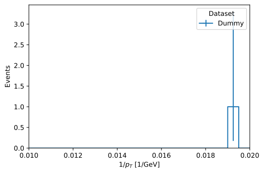
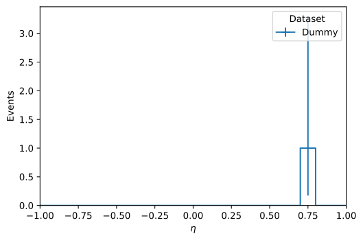
Notice how integrate can be used to reduce the dimensions of a histograms. You can also provide a custom integration range if you want to perform additional selections on binned dataset. Also

hist.plot1d(output['hist'].integrate('invpt', slice(0.015,0.020)))

<AxesSubplot:xlabel='$\\eta$', ylabel='Events'>

Scaling up calculations – process executors

Suppose you have some file set, you can define coffea to run over all file with a given metadata tag using the following

output = processor.run_uproot_job(
    {
        'Dataset1': ['TTbar.root'],
        'Dataset2': ['TTbar.root', 'TTbar.root']
    },
    treename="Events",
    processor_instance=DummyProcessor(),
    executor=processor.futures_executor,
    executor_args={"schema": NanoAODSchema, "workers": 10},
)

Now at first glance this seems to be a very straight forwards translation to the form what we already have in the NanoEventsFractory method. The magic statement that give coffea simple scalability is the use of the executor argument. By using the processor.futures_executor, you have already enabled local multithreading with a maximum of 10 parallel threads, by doing so, we have just showed through nearly 10 gigabytes of data in less than 5 seconds! Aside from the futures_executor. There is also the iterative_executor for single thread processing, which is the best for analysis debugging, since parallelism would cause the error messages to be wrapped in additional thread-related messages. There is also the dask_executor, which submits job to the grid computing resource available to machine running the notebook. If you already have the settings stored somewhere on, you can switch from a debugging to grid-level parallel programming simply by changing a couple of lines in the notebook! Examples of the configuration required to run grid-level parallelism can be found in the example snippets.

A couple of notes on how parallelism works on the various executors: it is still file-based (i.e. each file generates their own events awkward array to be processed), so be careful that when running the futures_executor during moderate testing you don’t saturate memory usage of your local machine. Because of this, if you create a histogram to keep a tally of len(events), what you would get is not a single number of events for each sample, but rather the various number of events stored in each file. While it might be conceptually helpful to think abstractly that the input events object to the process method is a massive awkward array that spans the entire data set, this is not how the processor is actually working.

Also, now we can comment on how process accumulator are performed across multiple jobs. The contents of each of the accumulator instances are added together via the __sum__ operator. For coffea.hist histogram, this method is already overloaded to behave how one would expect histogram aggregation to work, but you can supply your own class with the __sum__ operator overloaded if you really want. Right now, there is no standard class to aggregate unbinned data, since the unbinned data can be arbitrarily large, so in a grid-level computation settings one would want to keep the unbinned data on each worker node until they are called by the main thread for further processing, as returning all data to the main thread will likely saturate all resources on a single machine. The core developers are currently working on this general use case which uses a different data format, but if you know that your final output data frame is expected to be small (ex you have a very tight background rejection selection), you can write your own accumulator class to get unbinned data.